Indirect Data Analysis
The Indirect Data Analysis interface is a collection of tools within MantidPlot
for analysing reduced data from indirect geometry spectrometers, such as IRIS and
OSIRIS.
The majority of the functions used within this interface can be used with both
reduced files (_red.nxs) and workspaces (_red) created using the Indirect Data
Reduction interface or using  files (_sqw.nxs) and
workspaces (_sqw) created using either the Indirect Data Reduction interface or
taken from a bespoke algorithm or auto reduction.
files (_sqw.nxs) and
workspaces (_sqw) created using either the Indirect Data Reduction interface or
taken from a bespoke algorithm or auto reduction.
Four of the available tabs are QENS fitting interfaces and share common features and
layout. These common factors are documented in the QENS Fitting Interfaces Features section of this document.
These interfaces do not support GroupWorkspace as input.
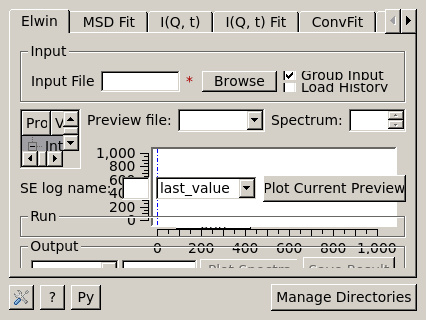
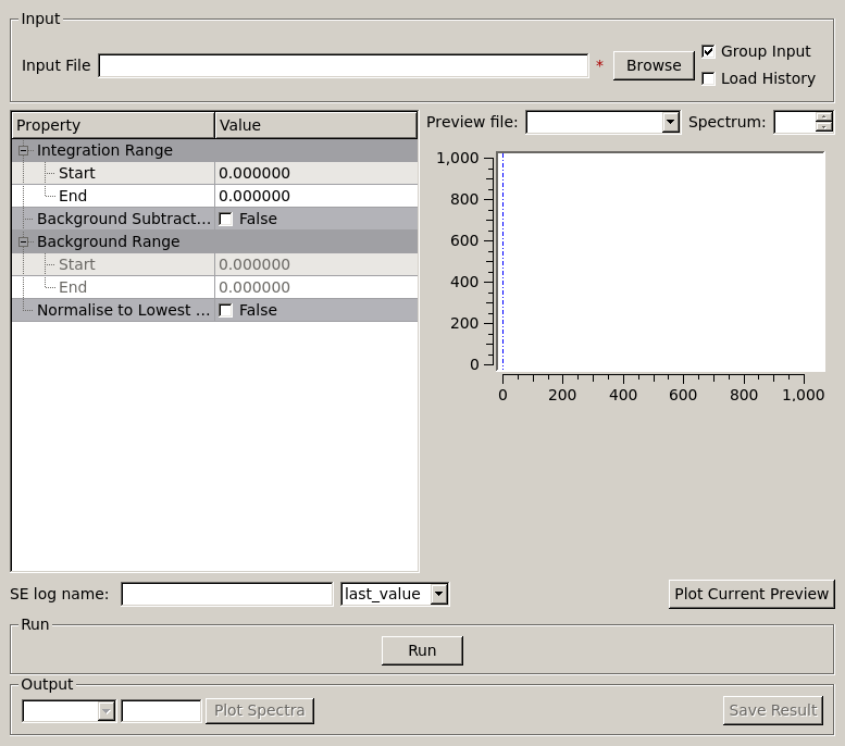
Provides an interface for the ElasticWindow
algorithm, with the option of selecting the range to integrate over as well as
the background range. An on-screen plot is also provided.
For workspaces that have a sample log or have a sample log file available in the
Mantid data search paths that contains the sample environment information the
ELF workspace can also be normalised to the lowest temperature run in the range
of input files.
- Input File
- Specify a range of input files that are either reduced (_red.nxs) or
.
- Group Input
- The ElasticWindowMultiple algorithm is performed on the input files and returns a group
workspace as the output. This option, if unchecked, will ungroup these output workspaces.
- Load History
- If unchecked the input workspace will be loaded without it’s history.
- Integration Range
- The energy range over which to integrate the values.
- Background Subtraction
- If checked a background will be calculated and subtracted from the raw data.
- Background Range
- The energy range over which a background is calculated which is subtracted from
the raw data.
- Normalise to Lowest Temp
- If checked the raw files will be normalised to the run with the lowest
temperature, to do this there must be a valid sample environment entry in the
sample logs for each of the input files.
- SE log name
- The name of the sample environment log entry in the input files sample logs
(defaults to ‘sample’).
- SE log value
- The value to be taken from the “SE log name” data series (defaults to the
specified value in the instrument parameters file, and in the absence of such
specification, defaults to “last value”)
- Preview File
- The workspace currently active in the preview plot.
- Spectrum
- Changes the spectrum displayed in the preview plot.
- Plot Current Preview
- Plots the currently selected preview plot in a separate external window
- Run
- Runs the processing configured on the current tab.
- Plot Spectra
- If enabled, it will plot the selected workspace indices in the selected output workspace.
- Save Result
- Saves the result in the default save directory.
The Elwin tab operates on _red and _sqw files. The files used in this workflow can
be produced using the run numbers 104371-104375 on the
Indirect Data Reduction interface in the ISIS Energy
Transfer tab. The instrument used to produce these files is OSIRIS, the analyser is graphite
and the reflection is 002.
- Untick the Load History checkbox next to the file selector if you want to load your data
without history.
- Click Browse and select the files osiris104371_graphite002_red,
osiris104372_graphite002_red, osiris104373_graphite002_red, osiris104374_graphite002_red
and osiris104375_graphite002_red. Load these files and they will be plotted in the mini-plot
automatically.
- The workspace and spectrum displayed in the mini-plot can be changed using the combobox and
spinbox seen directly above the mini-plot.
- You may opt to change the x range of the mini-plot by changing the Integration Range, or
by sliding the blue lines seen on the mini-plot using the cursor. For the purpose of this
demonstration, use the default x range.
- Tick Normalise to Lowest Temp. This option will produce an extra workspace with end suffix
_elt. However, for this to work the input workspaces must have a temperature. See the
description above for more information.
- Click Plot Current Preview if you want a larger plot of the mini-plot.
- Click Run and wait for the interface to finish processing. This should generate four
workspaces ending in _eq, _eq2, _elf and _elt.
- In the Output section, select the workspace ending with _eq and then choose some workspace
indices (e.g. 0-2,4). Click Plot Spectra to plot the spectrum from the selected workspace.
- Choose a default save directory and then click Save Result to save the output workspaces.
The workspace ending in _eq will be used in the MSD Fit Example Workflow.
Given either a saved NeXus file or workspace generated using the Elwin tab, this
tab fits  vs.
vs.  with one of three functions for each
run specified to give the Mean Square Displacement (MSD). It then plots the MSD
as function of run number. This is done by means of the
QENSFitSequential algorithm.
with one of three functions for each
run specified to give the Mean Square Displacement (MSD). It then plots the MSD
as function of run number. This is done by means of the
QENSFitSequential algorithm.
MSDFit searches for the log files named <runnumber>_sample.txt in your chosen
raw file directory (the name ‘sample’ is for OSIRIS). These log files will exist
if the correct temperature was loaded using SE-log-name in the Elwin tab. If they
exist the temperature is read and the MSD is plotted versus temperature; if they do
not exist the MSD is plotted versus run number (last 3 digits).
The fitted parameters for all runs are in _msd_Table and the <u2> in _msd. To
run the Sequential fit a workspace named <inst><first-run>_to_<last-run>_eq is
created of v. for all runs. A contour or 3D plot of
this may be of interest.
A sequential fit is run by clicking the Run button at the bottom of the tab, a
single fit can be done using the Fit Single Spectrum button underneath the
preview plot.
The Peters model [1] reduces to a Gaussian at large
(towards infinity) beta. The Yi Model [2] reduces to a Gaussian at sigma
equal to zero.
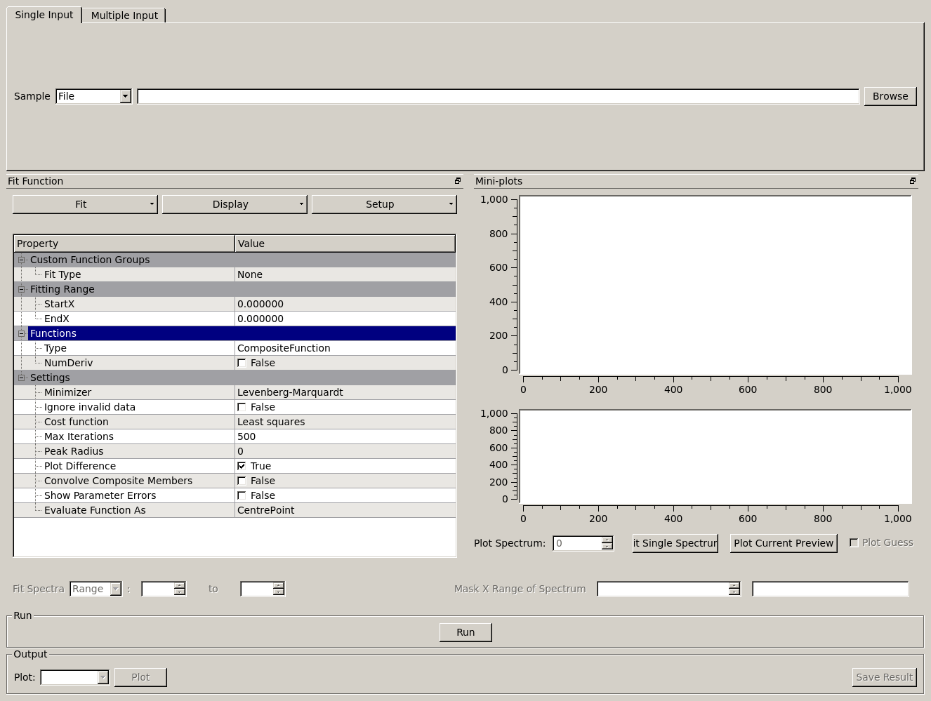
- Sample
- A file with extension _eq.nxs that has been created using the Elwin tab with an
 axis of
. Alternatively, a workspace may be provided.
axis of
. Alternatively, a workspace may be provided.
- Single Input/Multiple Input
- Choose between loading a single workspace or multiple workspaces.
- Function Browser
- This is used to decide the details of your fit including the fit type and minimizer used. It is
possible to un-dock this browser.
- Mini Plots
- The top plot displays the sample data, guess and fit. The bottom plot displays the difference between
the sample data and fit. It is possible to un-dock these plots.
- Plot Spectrum
- Changes the spectrum displayed in the mini plots.
- Fit Single Spectrum
- This will Fit a single spectrum selected by the neighboring Plot Spectrum spinbox.
- Plot Current Preview
- Plots the currently selected preview plot in a separate external window
- Plot Guess
- This will a plot a guess of your fit based on the information selected in the Function Browser.
- Fit Spectra
- Choose a range or discontinuous list of spectra to be fitted.
- Mask X Range
- Energy ranges may be excluded from a fit by selecting a spectrum next to the ‘Mask X Range of Spectrum’ label
and then providing a comma-separated list of pairs, where each pair designates a range to exclude from the fit.
- Run
- Runs the processing configured on the current tab.
- Plot
- Plots the selected parameter stored in the result workspace.
- Save Result
- Saves the workspaces from the _Results group workspace in the default save directory.
See also
Sequential fitting is available, options are detailed in the Sequential Fitting section.
The MSD Fit tab operates on _eq files. The files used in this workflow are produced on the Elwin
tab as seen in the Elwin Example Workflow.
- Click Browse and select the file osi104371-104375_graphite002_red_elwin_eq. Load this
file and it will be automatically plotted in the upper mini-plot.
- Change the Plot Spectrum spinbox seen underneath the mini-plots to change the spectrum displayed
in the upper mini-plot.
- Change the EndX variable to be around 0.8 in order to change the Q range over which the fit shall
take place. Alternatively, drag the EndX blue line seen on the mini-plot using the cursor.
- Choose the Fit Type to be Gaussian. The parameters for this function can be seen if you
expand the row labelled f0-MsdGauss. Choose appropriate starting values for these parameters.
It is possible to constrain one of the parameters by right clicking a parameter and selecting
Constrain.
- Tick Plot Guess to get a prediction of what your fit will look like.
- Click Run and wait for the interface to finish processing. This should generate a
_Parameters table workspace and two group workspaces with end suffixes _Results and
_Workspaces. The mini-plots should also update, with the upper plot displaying the
calculated fit and the lower mini-plot displaying the difference between the input data and the
fit.
- Alternatively, you can click Fit Single Spectrum to perform a fit only for the spectrum
currently displayed in the upper mini-plot. Do not click this for the purposes of this
demonstration.
- In the Output section, select the Msd parameter and then click Plot. This plots the
Msd parameter which can be found within the _Results group workspace.
Go to the I(Q, t) Example Workflow.
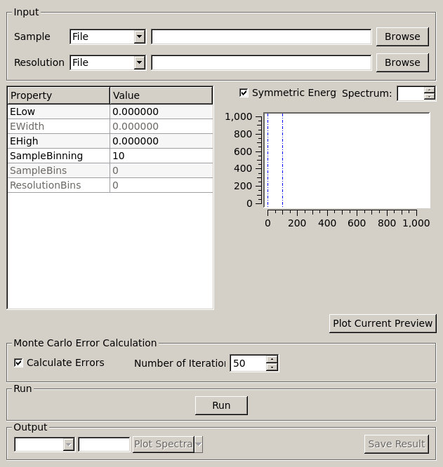
Given sample and resolution inputs, carries out a fit as per the theory detailed
in the TransformToIqt algorithm.
- Sample
- Either a reduced file (_red.nxs) or workspace (_red) or an
 file (_sqw.nxs) or workspace (_sqw).
- Resolution
- Either a resolution file (_res.nxs) or workspace (_res) or an file (_sqw.nxs) or workspace (_sqw).
- ELow, EHigh
- The rebinning range.
- SampleBinning
- The number of neighbouring bins are summed.
- Symmetric Energy Range
- Untick to allow an asymmetric energy range.
- Spectrum
- Changes the spectrum displayed in the preview plot.
- Plot Current Preview
- Plots the currently selected preview plot in a separate external window
- Calculate Errors
- The calculation of errors using a Monte Carlo implementation can be skipped by unchecking
this option.
- Number Of Iterations
- The number of iterations to perform in the Monte Carlo routine for error calculation
in I(Q,t).
- Run
- Runs the processing configured on the current tab.
- Plot Spectra
- If enabled, it will plot the selected workspace indices in the selected output workspace.
- Plot Tiled
- It will plot a tiled plot containing the selected workspace indices. It accessed via the down
arrow on the Plot Spectra button.
- Save Result
- Saves the result workspace in the default save directory.
The I(Q, t) tab allows _red and _sqw for it’s sample file, and allows _red, _sqw and
_res for the resolution file. The sample file used in this workflow can be produced using the run
number 26176 on the Indirect Data Reduction interface in the ISIS
Energy Transfer tab. The resolution file is created in the ISIS Calibration tab using the run number
26173. The instrument used to produce these files is IRIS, the analyser is graphite
and the reflection is 002.
- Click Browse for the sample and select the file iris26176_graphite002_red. Then click Browse
for the resolution and select the file iris26173_graphite002_res.
- Change the SampleBinning variable to be 5. Changing this will calculate values for the EWidth,
SampleBins and ResolutionBins variables automatically by using the
TransformToIqt algorithm where the BinReductionFactor is given by the
SampleBinning value. The SampleBinning value must be low enough for the ResolutionBins to be
at least 5. A description of this option can be found in the A note on Binning section.
- Untick Calculate Errors if you do not want to calculate the errors for the output workspace which
ends with the suffix _iqt.
- Click Run and wait for the interface to finish processing. This should generate a workspace ending
with a suffix _iqt.
- In the Output section, select some workspace indices (e.g.0-2,4,6) for a tiled plot and then click
the down arrow on the Plot Spectra button before clicking Plot Tiled.
- Choose a default save directory and then click Save Result to save the _iqt workspace.
This workspace will be used in the I(Q, t) Fit Example Workflow.
The bin width is determined by the energy range and the sample binning factor. The number of bins is automatically
calculated based on the SampleBinning specified. The width is determined by the width of the range divided
by the number of bins.
The following binning parameters are not enterable by the user and are instead automatically calculated through
the TransformToIqt algorithm once a valid resolution file has been loaded. The calculated
binning parameters are displayed alongside the binning options:
- EWidth
- The calculated bin width.
- SampleBins
- The number of bins in the sample after rebinning.
- ResolutionBins
- The number of bins in the resolution after rebinning. Typically this should be at
least 5 and a warning will be shown if it is less.
I(Q, t) Fit provides a simplified interface for controlling various fitting
functions (see the Fit algorithm for more info). The functions
are also available via the fit wizard.
The fit types available for use in IqtFit are Exponentials and
Stretched Exponential.
- Sample
- Either a file (_iqt.nxs) or workspace (_iqt) that has been created using
the Iqt tab.
- Single Input/Multiple Input
- Choose between loading a single workspace or multiple workspaces.
- Function Browser
- This is used to decide the details of your fit including the fit type and minimizer used. Further options
are seen below. It is possible to un-dock this browser.
- Constrain Intensities
- Check to ensure that the sum of the background and intensities is always equal
to 1.
- Make Beta Global
- Check to use a multi-domain fitting function with the value of beta
constrained - the IqtFitSimultaneous will be
used to perform this fit.
- Extract Members
- If checked, each individual member of the fit (e.g. exponential functions), will
be extracted.
- Mini Plots
- The top plot displays the sample data, guess and fit. The bottom plot displays the difference between
the sample data and fit. It is possible to un-dock these plots.
- Plot Spectrum
- Changes the spectrum displayed in the mini plots.
- Fit Single Spectrum
- This will Fit a single spectrum selected by the neighboring Plot Spectrum spinbox.
- Plot Current Preview
- Plots the currently selected preview plot in a separate external window
- Plot Guess
- This will a plot a guess of your fit based on the information selected in the Function Browser.
- Fit Spectra
- Choose a range or discontinuous list of spectra to be fitted.
- Mask X Range
- Energy ranges may be excluded from a fit by selecting a spectrum next to the ‘Mask X Range of Spectrum’ label
and then providing a comma-separated list of pairs, where each pair designates a range to exclude from the fit.
- Run
- Runs the processing configured on the current tab.
- Plot
- Plots the selected parameter stored in the result (or PDF) workspace.
- Edit Result
- Allows you to replace values within your _Results workspace using the IndirectReplaceFitResult
algorithm. See below for more detail.
- Save Result
- Saves the workspaces from the _Results group workspace in the default save directory.
See also
Sequential fitting is available, options are detailed in the Sequential Fitting section.
The I(Q, t) Fit tab operates on _iqt files. The files used in this workflow are produced on the
I(Q, t) tab as seen in the I(Q, t) Example Workflow.
- Click Browse and select the file irs26176_graphite002_iqt.
- Change the EndX variable to be around 0.2 in order to change the time range. Alternatively, drag
the EndX blue line seen on the upper mini-plot using the cursor.
- Choose the number of Exponentials to be 1. Select a Flat Background.
- Change the Fit Spectra to go from 0 to 7. This will ensure that only the spectra within the input
workspace with workspace indices between 0 and 7 are fitted.
- Click Run and wait for the interface to finish processing. This should generate a
_Parameters table workspace and two group workspaces with end suffixes _Results and
_Workspaces. The mini-plots should also update, with the upper plot displaying the
calculated fit and the lower mini-plot displaying the difference between the input data and the
fit.
- In the Output section, you can choose which parameter you want to plot.
- Click Fit Single Spectrum to produce a fit result for the first spectrum.
- In the Output section, click Edit Result and then select the _Result workspace containing
multiple fits (1), and in the second combobox select the _Result workspace containing the single fit
(2). Choose an output name and click Replace Fit Result. This will replace the corresponding fit result
in (1) with the fit result found in (2). See the IndirectReplaceFitResult
algorithm for more details. Note that the output workspace is inserted into the group workspace in which
(1) is found.
Go to the ConvFit Example Workflow.
ConvFit provides a simplified interface for controlling
various fitting functions (see the Fit algorithm for more
info). The functions are also available via the fit wizard.
Additionally, in the bottom-right of the interface there are options for doing a
sequential fit. This is where the program loops through each spectrum in the
input workspace, using the fitted values from the previous spectrum as input
values for fitting the next. This is done by means of the
ConvolutionFitSequential algorithm.
A sequential fit is run by clicking the Run button at the bottom of the tab, a
single fit can be done using the Fit Single Spectrum button underneath the
preview plot.
The fit types available in ConvFit are One Lorentzian, Two Lorentzian,
TeixeiraWater (SQE), InelasticDiffSphere,
InelasticDiffRotDiscreteCircle, ElasticDiffSphere,
ElasticDiffRotDiscreteCircle and StretchedExpFT.
See also
Sequential fitting is available, options are detailed in the Sequential Fitting section.
- Sample
- Either a reduced file (_red.nxs) or workspace (_red) or an file (_sqw.nxs, _sqw.dave) or workspace (_sqw).
- Resolution
- Either a resolution file (_res.nxs) or workspace (_res) or an file (_sqw.nxs, _sqw.dave) or workspace (_sqw).
- Single Input/Multiple Input
- Choose between loading a single workspace or multiple workspaces.
- Function Browser
- This is used to decide the details of your fit including the fit type and minimizer used. Further options
are seen below. It is possible to un-dock this browser.
- Use Delta Function
- Found under ‘Custom Function Groups’. Enables use of a delta function.
- Extract Members
- If checked, each individual member of the fit (e.g. exponential functions), will
be extracted into a <result_name>_Members group workspace.
- Use Temperature Correction
- Adds the custom user function for temperature correction to the fit function.
- Background Options
- Flat Background: Adds a flat background to the composite fit function. Linear Background: Adds a linear
background to the composite fit function.
- Mini Plots
- The top plot displays the sample data, guess and fit. The bottom plot displays the difference between
the sample data and fit. It is possible to un-dock these plots.
- Plot Spectrum
- Changes the spectrum displayed in the mini plots.
- Fit Single Spectrum
- This will Fit a single spectrum selected by the neighboring Plot Spectrum spinbox.
- Plot Current Preview
- Plots the currently selected preview plot in a separate external window
- Plot Guess
- This will a plot a guess of your fit based on the information selected in the Function Browser.
- Fit Spectra
- Choose a range or discontinuous list of spectra to be fitted.
- Mask X Range
- Energy ranges may be excluded from a fit by selecting a spectrum next to the ‘Mask X Range of Spectrum’ label
and then providing a comma-separated list of pairs, where each pair designates a range to exclude from the fit.
- Run
- Runs the processing configured on the current tab.
- Plot
- Plots the selected parameter stored in the result (or PDF) workspace.
- Edit Result
- Allows you to replace values within your _Results workspace using the IndirectReplaceFitResult
algorithm. See below for more detail.
- Save Result
- Saves the workspaces from the _Results group workspace in the default save directory.
The Conv Fit tab allows _red and _sqw for its sample file, and allows _red, _sqw and
_res for the resolution file. The sample file used in this workflow can be produced using the run
number 26176 on the Indirect Data Reduction interface in the ISIS
Energy Transfer tab. The resolution file is created in the ISIS Calibration tab using the run number
26173. The instrument used to produce these files is IRIS, the analyser is graphite
and the reflection is 002.
- Click Browse for the sample and select the file iris26176_graphite002_red. Then click Browse
for the resolution and select the file iris26173_graphite002_res.
- Choose the Fit Type to be One Lorentzian. Tick the Delta Function checkbox. Set the background
to be a Flat Background.
- Expand the variables called f0-Lorentzian and f1-DeltaFunction. To tie the delta functions Centre
to the PeakCentre of the Lorentzian, right click on the Centre parameter and go to Tie->Custom Tie and then
enter f0.PeakCentre.
- Tick Plot Guess to get a prediction of what your fit will look like.
- Click Run and wait for the interface to finish processing. This should generate a
_Parameters table workspace and two group workspaces with end suffixes _Results and
_Workspaces. The mini-plots should also update, with the upper plot displaying the
calculated fit and the lower mini-plot displaying the difference between the input data and the
fit.
- Choose a default save directory and then click Save Result to save the _result workspaces
found inside of the group workspace ending with _Results. The saved workspace will be used in
the F(Q) Fit Example Workflow.
For more on the theory of Conv Fit see the Conv Fit concept page.
One of the models used to interpret diffusion is that of jump diffusion in which
it is assumed that an atom remains at a given site for a time  ; and
then moves rapidly, that is, in a time negligible compared to .
; and
then moves rapidly, that is, in a time negligible compared to .
This interface can be used for a jump diffusion fit as well as fitting across
EISF. This is done by means of the
QENSFitSequential algorithm.
The fit types available in F(Q)Fit are ChudleyElliot, HallRoss,
FickDiffusion, TeixeiraWater, EISFDiffCylinder,
EISFDiffSphere and EISFDiffSphereAlkyl.
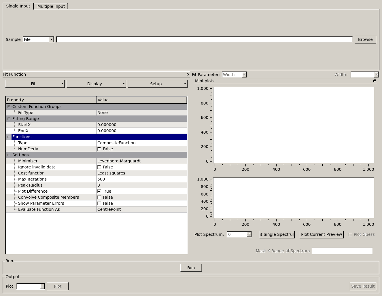
- Sample
- A sample workspace created with either ConvFit or Quasi.
- Single Input/Multiple Input
- Choose between loading a single workspace or multiple workspaces.
- Fit Parameter
- This allows you to select the type of parameter displayed in the neighbouring combobox to its right (see option below).
The allowed types are ‘Width’ and ‘EISF’. Changing this combobox will also change the available Fit types in the Function
Browser.
- Width/EISF
- Next to the ‘Fit Parameter’ menu, will be either a ‘Width’ or ‘EISF’ menu, depending on which was selected.
This menu can be used to select the specific width/EISF parameter to be fit. Selecting one of these parameters will automatically
set the active spectrum index of the loaded workspace in which this parameter is located.
- Function Browser
- This is used to decide the details of your fit including the fit type and minimizer used. Further options
are seen below. It is possible to un-dock this browser.
- Mini Plots
- The top plot displays the sample data, guess and fit. The bottom plot displays the difference between
the sample data and fit. It is possible to un-dock these plots.
- Plot Spectrum
- Changes the spectrum displayed in the mini plots.
- Fit Single Spectrum
- This will Fit a single spectrum selected by the neighboring Plot Spectrum spinbox.
- Plot Current Preview
- Plots the currently selected preview plot in a separate external window
- Plot Guess
- This will a plot a guess of your fit based on the information selected in the Function Browser.
- Fit Spectra
- Choose a range or discontinuous list of spectra to be fitted.
- Mask X Range
- Energy ranges may be excluded from a fit by selecting a spectrum next to the ‘Mask X Range of Spectrum’ label
and then providing a comma-separated list of pairs, where each pair designates a range to exclude from the fit.
- Run
- Runs the processing configured on the current tab.
- Plot
- Plots the selected parameter stored in the result workspace.
- Save Result
- Saves the workspaces from the _Results group workspace in the default save directory.
The F(Q) Fit tab operates on _result files which can be produced on the ConvFit tab. The
sample file used in this workflow is produced on the Conv Fit tab as seen in the
ConvFit Example Workflow.
- Click Browse and select the file irs26176_graphite002_conv_Delta1LFitF_s0_to_9_Result.
- Change the mini-plot data by choosing the type of Fit Parameter you want to display. For the
purposes of this demonstration select EISF. The combobox immediately to the right can be used to
choose which EISF you want to see in the mini-plot. In this example there is only one available.
- Change the Fit Parameter back to Width.
- Choose the Fit Type to be TeixeiraWater.
- Click Run and wait for the interface to finish processing. This should generate a
_Parameters table workspace and two group workspaces with end suffixes _Results and
_Workspaces. The mini-plots should also update, with the upper plot displaying the
calculated fit and the lower mini-plot displaying the difference between the input data and the
fit.
- In the Output section, you can choose which parameter you want to plot. In this case the plotting
option is disabled as the output workspace ending in _Result only has one data point to plot.
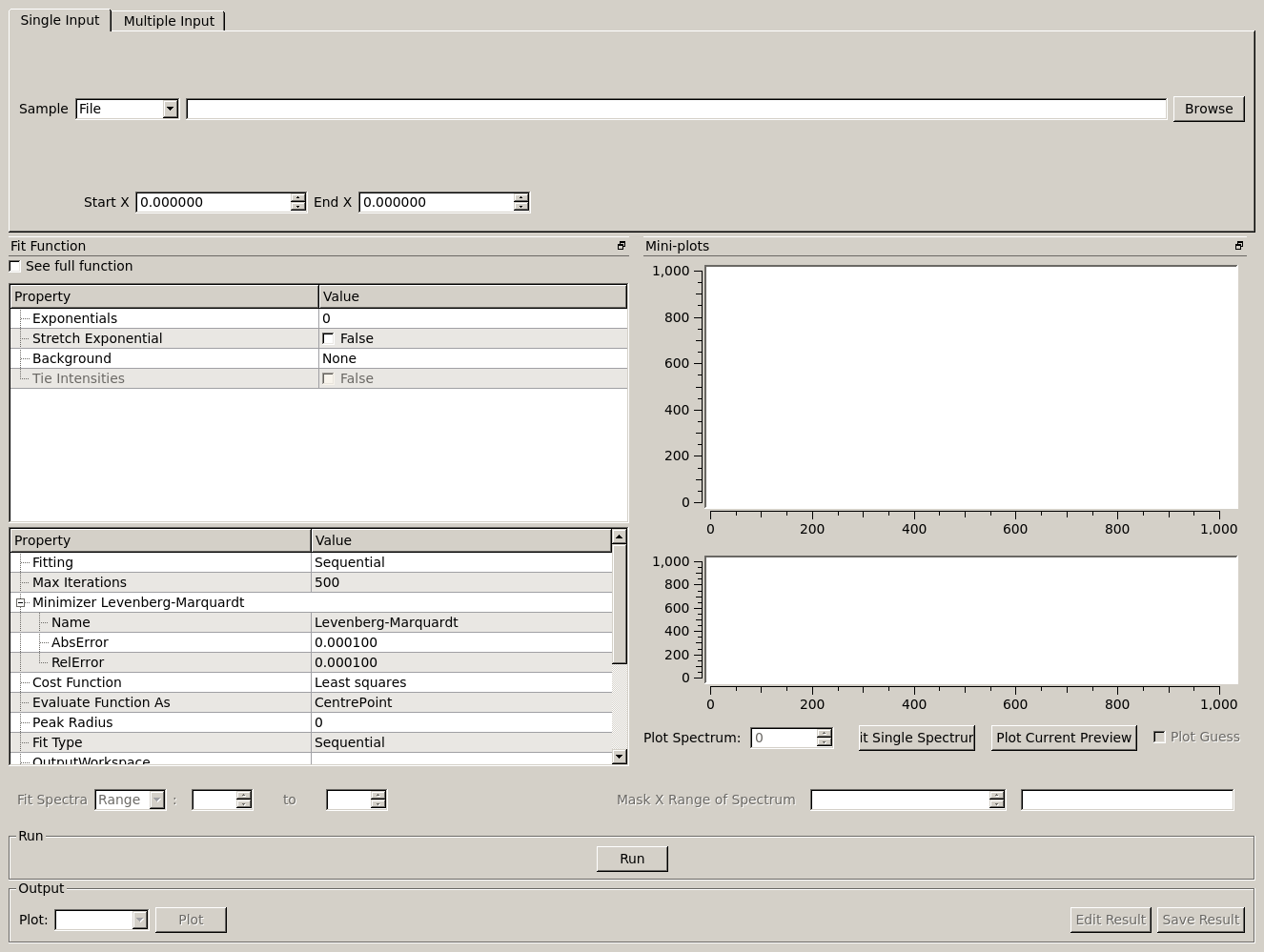
There are four QENS fitting interfaces:
- MSD Fit
- I(Q,t) Fit,
- Conv Fit
- F(Q)
These fitting interfaces share common features, with a few unique options in each.
Under ‘Custom Function Groups’, you will find utility options for quick selection of common fit functions, specific
to each fitting interface.
The ‘Fit Type’ drop-down menu will be available here in each of the QENS fitting interfaces – which is useful for
selecting common fit functions but not mandatory.
Under ‘Fitting Range’, you may select the start and end -values (‘StartX’ and ‘EndX’) to be used in the fit.
Under ‘Functions’, you can view the selected model and associated parameters as well as make modifications.
Right-clicking on ‘Functions’ and selecting ‘Add Function’ will allow you to add any function from Mantid’s library
of fitting functions. It is also possible to right-click on a composite function and select ‘Add Function’ to add a
function to the composite.
Parameters may be tied by right-clicking on a parameter and selecting either ‘Tie > To Function’ when creating a tie
to a parameter of the same name in a different function or by selecting ‘Tie > Custom Tie’ to tie to parameters of
different names and for providing mathematical expressions. Parameters can be constrained by right-clicking and
using the available options under ‘Constrain’.
Upon performing a fit, the parameter values will be updated here to display the result of the fit for the selected
spectrum.
- Minimizer
- The minimizer which will be used in the fit (defaults to Levenberg-Marquadt).
- Ignore invalid data
- Whether to ignore invalid (infinity/NaN) values when performing the fit.
- Cost function
- The cost function to be used in the fit (defaults to Least Squares).
- Max Iterations
- The maximum number of iterations used to perform the fit of each spectrum.
Two preview plots are included in each of the fitting interfaces. The top preview plot displays the sample, guess
and fit curves. The bottom preview plot displays the difference curve.
The preview plots will display the curves for the selected spectrum (‘Plot Spectrum’) of the selected data-set
(when in multiple input mode, a drop-down menu will be available above the plots to select the active data-set).
The ‘Plot Spectrum’ option can be used to select the active/displayed spectrum.
A button labelled ‘Fit Single Spectrum’ is found under the preview plots and can be used to perform a fit of the
selected specturm.
‘Plot Current Preview’ can be used to plot the sample, fit and difference curves of the selected spectrum in
a separate plotting window.
The ‘Plot Guess’ check-box can be used to enable/disable the guess curve in the top preview plot.
The results of the fit may be plotted and saved under the ‘Output’ section of the fitting interfaces.
Next to the ‘Plot’ label, you can select a parameter to plot and then click ‘Plot’ to plot it with error
bars across the fit spectra (if multiple data-sets have been used, a separate plot will be produced for each data-set).
The ‘Plot Output’ options will be disabled after a fit if there is only one data point for the parameters.
During a sequential fit, the parameters calculated for one spectrum become the start parameters for the next spectrum to be fitted.
Although this normally yields better parameter values for the later spectra, it can also lead to poorly fitted parameters if the
next spectrum is not ‘related’ to the previous spectrum. It may be useful to replace this poorly fitted spectrum with the results
from a single fit using the ‘Edit Result’ option.
Clicking the ‘Edit Result’ button will allow you to modify the data within your _Results workspace using results
produced from a singly fit spectrum. See the algorithm IndirectReplaceFitResult.
Clicking the ‘Save Result’ button will save the result of the fit to your default save location.
There is the option to perform Bayesian data analysis on the I(Q, t) Fit ConvFit
tabs on this interface by using the FABADA fitting minimizer, however in
order to to use this you will need to use better starting parameters than the
defaults provided by the interface.
You may also experience issues where the starting parameters may give a reliable
fit on one spectra but not others, in this case the best option is to reduce
the number of spectra that are fitted in one operation.
In both I(Q, t) Fit and ConvFit the following options are available when fitting
using FABADA:
- Output Chain
- Select to enable output of the FABADA chain when using FABADA as the fitting
minimizer.
- Chain Length
- Number of further steps carried out by fitting algorithm once parameters have
converged (see ChainLength is FABADA documentation)
- Convergence Criteria
- The minimum variation in the cost function before the parameters are
considered to have converged (see ConvergenceCriteria in FABADA
documentation)
- Acceptance Rate
- The desired percentage acceptance of new parameters (see JumpAcceptanceRate
in FABADA documentation)
The FABADA minimizer can output a PDF group workspace when the PDF option is ticked. If this happens,
then it is possible to plot this PDF data using the output options at the bottom of the tabs.
Three of the fitting interfaces allow sequential fitting of several spectra:
- MSD Fit
- I(Q, T) Fit
- ConvFit
At the bottom of the interface there are options for doing a
sequential fit. This is where the program loops through each spectrum in the
input workspace, using the fitted values from the previous spectrum as input
values for fitting the next. This is done by means of the
IqtFitSequential algorithm.
A sequential fit is run by clicking the Run button seen just above the output
options, a single fit can be done using the Fit Single Spectrum button underneath
the preview plot.
Below the preview plots, the spectra to be fit can be selected. The ‘Fit Spectra’ drop-down menu allows for
selecting either ‘Range’ or ‘String’. If ‘Range’ is selected, you are able to select a range of spectra to fit by
providing the upper and lower bounds. If ‘String’ is selected you can provide the spectra to fit in a text form.
When selecting spectra using text, you can use ‘-‘ to identify a range and ‘,’ to separate each spectrum/range.
 -Ranges may be excluded from the fit by selecting a spectrum next to the ‘Mask Bins of Spectrum’ label and
then providing a comma-separated list of pairs, where each pair designates a range to exclude from the fit.
-Ranges may be excluded from the fit by selecting a spectrum next to the ‘Mask Bins of Spectrum’ label and
then providing a comma-separated list of pairs, where each pair designates a range to exclude from the fit.
The model used to perform fitting in ConvFit is described in the following tree, note that
everything under the Model section is optional and determined by the Fit Type
and Use Delta Function options in the interface.
The Temperature Correction is a UserFunction with the
formula  where
where
 is the temperature in Kelvin.
References
- Peters & Kneller, Journal of Chemical Physics, 139, 165102 (2013)
- Yi et al, J Phys Chem B 116, 5028 (2012)
Categories: Interfaces | Indirect